Setup and execute DustPOL-py

1 Installation

1-Download the source files from: github

2-Go to the directory

3-From the terminal, type

pip install -e .

It is recommended to use a virtual environment to prevent conflicts with existing Python packages.

2 Physical Parameters

The basic physical parameters for DustPOL-py are listed as below

Parameter	Example Value	Comments
output_dir	output	directory for the outputs
ratd	off	turn on/off rotational disruption
U	3.0	radiation field (dimensionless)
gamma	0.3	anisotropic degree of radiation field
mean_lam	1.3	mean wavelength of radiation field
d	0
ngas	1.4e5	gas volume density (cm-3)
Tgas	16.4	gas temperature (K)
aligned_dust	astro	‘sil’ or ‘car’ or ‘sil+car’ or ‘astro’
amin	3.1e-4	mininum grain size (micron)
amax	1.0	maximum grain size (micron)
Tdust	0	dust temperature (K)
		* 0: convert U to Tdust
		* numerics: convert Tdust to U when U=0
rho	3	[g*cm^-3]:dust volume density
alpha	1.4	grain axes-ratio #prolate 0.3333
Smax	1e7	[erg cm-3]: tensile strength of grains
		*effective only when ratd=‘on’
dust_gas_ratio	0.01	dust-to-gas-mass ratio
law	MRN	size-distribution law: ‘MRN’ or ‘WD01’ or ‘DL07’
power_index	-3.5	power-index of GSD if ‘MRN’
RATalign	RAT	RAT or MRAT theory
fmax	1.0	1=100%: maximum of grain alignment efficiency
Bfield	600.0	strength of B-field (only active for MRAT)
B_angle	90.0	[deg] inclination angle of B-field wrt. LOS
Ncl	10.	if RATalign==MRAT (Ncl: number of iron atoms per cluster)
phi_sp	0.1	volume fitting factor of iron cluster (0.1=10%)
fp	0.1	Iron fraction of PM grains
parallel	True	Parallelization calculation for heavily computed tasked
cpu	-1	if parallel is used, give the number of cpu cores (-1 means all)

3 Run simple model (0D)

Let’s download the input physical parameters (Download) and save it in an sub-folder ‘data’ from your directory (the name is default as ‘input_template.dustpol’, but you are encouraged to rename it).

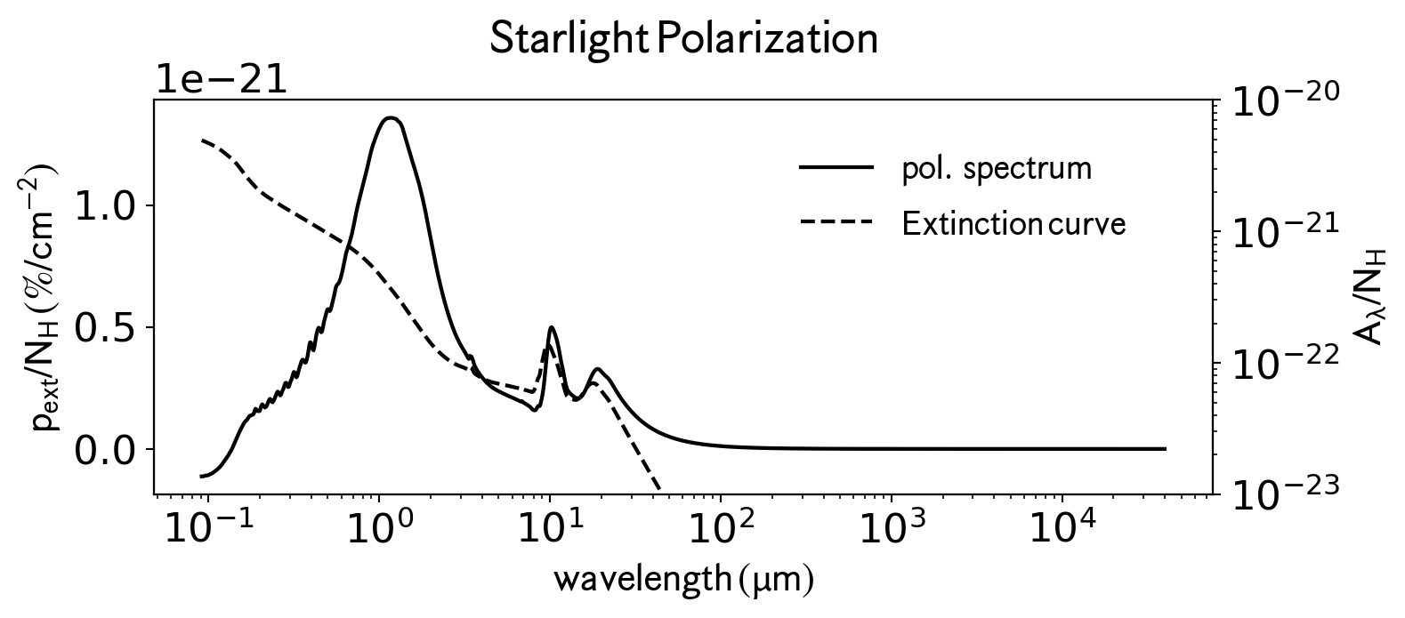
3.1 Starlight polarization

Here is a simple example showing how to compute the starlight polarisation (see Figure 1) for \(n_{\rm gas}=1.4\times 10^{5}\,\rm cm^{-3}\), \(U=3\), \(\bar{\lambda}=1.3\,\mu\)m and \(a_{\rm max}=1\,\mu\)m. DustPOL-py is called as

import matplotlib.pyplot as plt
from DustPOL_py import DustPOL
exe = DustPOL('data/input_template.dustpol') 
w,pext,_=exe.cal_pol_abs()
ext_curve = exe.extinction()

fig, ax = plt.subplots(figsize=(8, 3))
ax.set_xlabel('$\\rm wavelength\\,(\\mu m)$')
ax.set_ylabel('$\\rm p_{ext}/N_{H}\\,(\\%/cm^{-2})$')
ax.set_title('$\\rm Starlight\\,Polarization$',pad=20)
ax1=ax.twinx()
ax1.set_ylabel('$\\rm A_{\\lambda}/N_{\\rm H}$')

ax.semilogx(w * 1e4, pext/exe.ngas,color='k',ls='-')
ax1.loglog(w * 1e4, ext_curve,color='k',ls='--')
                 
ax1.loglog([],[],color='k',ls='-',label='$\\rm pol.\\,spectrum$')
ax1.loglog([],[],color='k',ls='--',label='$\\rm Extinction\\, curve$')
ax1.legend(bbox_to_anchor=(0.95,0.95),frameon=False)
ax1.set_ylim([1e-23,1e-20])

plt.show()

      U=3.000            
INFO:  ---> ngas=1.400e+05 (cm-3), amin=3.162e-04 (um), amax=0.531 (um), a_ali=0.183 (um), f_max=1.000, Tgas=16.400 (K), mean_lam=1.300 (um)         [DustPOL_py.align]

Figure 1: An example of polarisation spectrum for starlight dust polarisation

Note: to save output, use exe.cal_pol_abs(save_output=True). The output will be named as starlight.dat

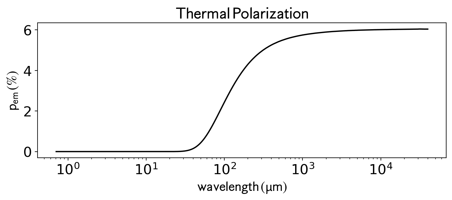
3.2 Thermal dust polarization

Using the same input parameters as above, here is a simple example showing how to compute the thermal dust polarisation (see Figure 2), DustPOL-py is called as

import matplotlib.pyplot as plt
from DustPOL_py import DustPOL
w,I_list,p_list=DustPOL('data/input_template.dustpol').cal_pol_emi()
fig,ax=plt.subplots(figsize=(9,3))
ax.semilogx(w*1e4,p_list[0],color='k',ls='-')
ax.set_xlabel('$\\rm wavelength\\,(\\mu m)$')
ax.set_ylabel('$\\rm p_{em}\\,(\\%)$')
ax.set_title('$\\rm Thermal\\,Polarization$')
plt.show()

INFO:  U=3.000 : radiation -->> Tdust             [DustPOL_py.DustPOL_class]
INFO:  ---> ngas=1.400e+05 (cm-3), amin=3.162e-04 (um), amax=0.531 (um), a_ali=0.183 (um), f_max=1.000, Tgas=16.400 (K), mean_lam=1.300 (um)         [DustPOL_py.align]

Figure 2: An example of polarisation spectrum for thermal dust polarisation

Note: to save output, use cal_pol_emi(save_output=True). The output will be named as thermal.dat

4 Run a 1D model

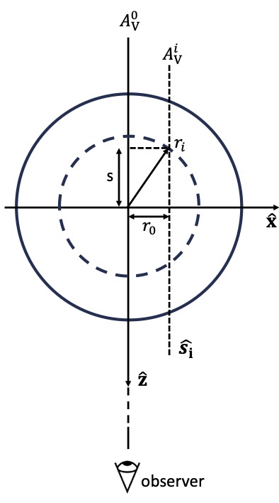
Descriptive Text — Figure 3: Coordinate system of the isolated cloud on the {}-plane with the \({\hat{z}}\) direction towards the observer. The position in the plane of the sky is defined by \(r_{0}\). Each line of sight \(\hat{s}\) corresponds to a distinct visual extinction \(A_{\rm V}\), calculated due to the gas volume density profile along this direction.

For the recent version of the model, an isolated cloud with a spherical geometry is adopted. To utilize this module, you must provide the profile of the gas volume density. For an example, let us compute the polarization degree along a line of sight through a peak gas density. In the coordinate system defined in Figure 3, \(r_{0}=0\). With this option, addition physical parameters are required

Parameter	Example Value	Comments
p	2	power-index for profiling gas volume density (n~r^-p)
rin	1700.	[au]: inner radius
rout	1.248e5	[au]: outer radius
rflat	9000.	[au]: flat radius (r<r0: n=n0=const.), while r>r0: n~r^{-p}
nsample	70	number of points sampling from rin -> rout

These parameters must be adjusted for different target.

isoCloud_los

import matplotlib.pyplot as plt
from DustPOL_py import DustPOL
exe = DustPOL('data/input_template.dustpol')
exe.isoCloud_los(0.0,progress=True,save_output=True)

As we can recognize, for other lines of sight, just simply pass the corresponding value of \(r_{0}\). The results can be written out when needed. To monitor the variations of the physical parameters, set progress=False

5 Run a 2D model

For an isolated spherical cloud/core illustrated in Figure 3, one can model the degree of dust polarization on the plane-of-sky by varying the values of \(r_{0}\) from center (\(0\)) to the edge of the cloud/core (\(r_{\rm out}\)). Typically, this task is time-consuming; thus we adopt the concurrency technique in python for parallelization. The setup is adjustable in the physical parameters input file. In DustPOL-py, this sight line coordinate is automically varied within the setup of the model, so we can just call this module

isoCloud_pos

import matplotlib.pyplot as plt
from DustPOL_py import DustPOL
exe = DustPOL('data/input_template.dustpol')
exe.isoCloud_pos()

The outputs are automatically written out. See the Examples/Scripts for an example.